Tissue Classification of a T1-weighted Structural Image

This example explains how to segment a T1-weighted structural image by using Bayesian formulation. The observation model (likelihood term) is defined as a Gaussian distribution and a Markov Random Field (MRF) is used to model the a priori probability of context-dependent patterns of different tissue types of the brain. Expectation Maximization and Iterated Conditional Modes are used to find the optimal solution. Similar algorithms have been proposed by Zhang et al. [Zhang2001] and Avants et al. [Avants2011] available in FAST-FSL and ANTS-atropos, respectively.

Here we will use a T1-weighted image, that has been previously skull-stripped and bias field corrected.

import numpy as np
import matplotlib.pyplot as plt
from dipy.data import get_fnames
from dipy.io.image import load_nifti_data
from dipy.segment.tissue import TissueClassifierHMRF
import time

First we fetch the T1 volume from the Syn dataset and determine its shape.

t1_fname, _, _ = get_fnames('tissue_data')
t1 = load_nifti_data(t1_fname)
print('t1.shape (%d, %d, %d)' % t1.shape)

t1.shape (256, 256, 176)

We have fetched the T1 volume. Now we will look at the axial and coronal slices of the image.

fig = plt.figure()
a = fig.add_subplot(1, 2, 1)
img_ax = np.rot90(t1[..., 89])
imgplot = plt.imshow(img_ax, cmap="gray")
a.axis('off')
a.set_title('Axial')
a = fig.add_subplot(1, 2, 2)
img_cor = np.rot90(t1[:, 128, :])
imgplot = plt.imshow(img_cor, cmap="gray")
a.axis('off')
a.set_title('Coronal')
plt.savefig('t1_image.png', bbox_inches='tight', pad_inches=0)

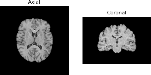
T1-weighted image of healthy adult.

Now we will define the other two parameters for the segmentation algorithm. We will segment three classes, namely corticospinal fluid (CSF), white matter (WM) and gray matter (GM).

nclass = 3

Then, the smoothness factor of the segmentation. Good performance is achieved with values between 0 and 0.5.

beta = 0.1

We could also set the number of iterations. By default this parameter is set to 100 iterations, but most of the time the ICM (Iterated Conditional Modes) loop will converge before reaching the 100th iteration. After setting the necessary parameters we can now call an instance of the class “TissueClassifierHMRF” and its method called “classify” and input the parameters defined above to perform the segmentation task.

Now we plot the resulting segmentation.

t0 = time.time()

hmrf = TissueClassifierHMRF()
initial_segmentation, final_segmentation, PVE = hmrf.classify(t1, nclass, beta)

t1 = time.time()
total_time = t1-t0
print('Total time:' + str(total_time))

fig = plt.figure()
a = fig.add_subplot(1, 2, 1)
img_ax = np.rot90(final_segmentation[..., 89])
imgplot = plt.imshow(img_ax)
a.axis('off')
a.set_title('Axial')
a = fig.add_subplot(1, 2, 2)
img_cor = np.rot90(final_segmentation[:, 128, :])
imgplot = plt.imshow(img_cor)
a.axis('off')
a.set_title('Coronal')
plt.savefig('final_seg.png', bbox_inches='tight', pad_inches=0)

>> Iteration: 0
>> Iteration: 1
>> Iteration: 2
>> Iteration: 3
>> Iteration: 4
>> Iteration: 5
>> Iteration: 6
>> Iteration: 7
>> Iteration: 8
>> Iteration: 9
>> Iteration: 10
>> Iteration: 11
>> Iteration: 12
>> Iteration: 13
>> Iteration: 14
>> Iteration: 15
>> Iteration: 16
>> Iteration: 17
>> Iteration: 18
>> Iteration: 19
>> Iteration: 20
Total time:176.59300875663757

Each tissue class is color coded separately, red for the WM, yellow for the GM and light blue for the CSF.

And we will also have a look at the probability maps for each tissue class.

fig = plt.figure()
a = fig.add_subplot(1, 3, 1)
img_ax = np.rot90(PVE[..., 89, 0])
imgplot = plt.imshow(img_ax, cmap="gray")
a.axis('off')
a.set_title('CSF')
a = fig.add_subplot(1, 3, 2)
img_cor = np.rot90(PVE[:, :, 89, 1])
imgplot = plt.imshow(img_cor, cmap="gray")
a.axis('off')
a.set_title('Gray Matter')
a = fig.add_subplot(1, 3, 3)
img_cor = np.rot90(PVE[:, :, 89, 2])
imgplot = plt.imshow(img_cor, cmap="gray")
a.axis('off')
a.set_title('White Matter')
plt.savefig('probabilities.png', bbox_inches='tight', pad_inches=0)
plt.show()

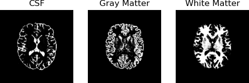
These are the probability maps of each of the three tissue classes.

References

[Zhang2001]

Zhang, Y., Brady, M. and Smith, S. Segmentation of Brain MR Images Through a Hidden Markov Random Field Model and the Expectation-Maximization Algorithm IEEE Transactions on Medical Imaging, 20(1): 45-56, 2001

[Avants2011]

Avants, B. B., Tustison, N. J., Wu, J., Cook, P. A. and Gee, J. C. An open source multivariate framework for n-tissue segmentation with evaluation on public data. Neuroinformatics, 9(4): 381-400, 2011.