DKI MultiTensor Simulation

In this example we show how to simulate the Diffusion Kurtosis Imaging (DKI) data of a single voxel. DKI captures information about the non-Gaussian properties of water diffusion which is a consequence of the existence of tissue barriers and compartments. In these simulations compartmental heterogeneity is taken into account by modeling different compartments for the intra- and extra-cellular media of two populations of fibers. These simulations are performed according to [RNH2015].

We first import all relevant modules.

import numpy as np
import matplotlib.pyplot as plt
from dipy.sims.voxel import (multi_tensor_dki, single_tensor)
from dipy.data import get_fnames
from dipy.io.gradients import read_bvals_bvecs
from dipy.core.gradients import gradient_table
from dipy.reconst.dti import (decompose_tensor, from_lower_triangular)

For the simulation we will need a GradientTable with the b-values and b-vectors. Here we use the GradientTable of the sample DIPY dataset small_64D.

fimg, fbvals, fbvecs = get_fnames('small_64D')
bvals, bvecs = read_bvals_bvecs(fbvals, fbvecs)

DKI requires data from more than one non-zero b-value. Since the dataset small_64D was acquired with one non-zero b-value we artificially produce a second non-zero b-value.

bvals = np.concatenate((bvals, bvals * 2), axis=0)
bvecs = np.concatenate((bvecs, bvecs), axis=0)

The b-values and gradient directions are then converted to DIPY’s GradientTable format.

gtab = gradient_table(bvals, bvecs)

In mevals we save the eigenvalues of each tensor. To simulate crossing fibers with two different media (representing intra and extra-cellular media), a total of four components have to be taken in to account (i.e. the first two compartments correspond to the intra and extra cellular media for the first fiber population while the others correspond to the media of the second fiber population)

mevals = np.array([[0.00099, 0, 0],
                   [0.00226, 0.00087, 0.00087],
                   [0.00099, 0, 0],
                   [0.00226, 0.00087, 0.00087]])

In angles we save in polar coordinates (\(\theta, \phi\)) the principal axis of each compartment tensor. To simulate crossing fibers at 70:math:^{circ} the compartments of the first fiber are aligned to the X-axis while the compartments of the second fiber are aligned to the X-Z plane with an angular deviation of 70:math:^{\circ} from the first one.

angles = [(90, 0), (90, 0), (20, 0), (20, 0)]

In fractions we save the percentage of the contribution of each compartment, which is computed by multiplying the percentage of contribution of each fiber population and the water fraction of each different medium

fie = 0.49  # intra-axonal water fraction
fractions = [fie*50, (1 - fie)*50, fie*50, (1 - fie)*50]

Having defined the parameters for all tissue compartments, the elements of the diffusion tensor (DT), the elements of the kurtosis tensor (KT) and the DW signals simulated from the DKI model can be obtain using the function multi_tensor_dki.

signal_dki, dt, kt = multi_tensor_dki(gtab, mevals, S0=200, angles=angles,
                                      fractions=fractions, snr=None)

We can also add Rician noise with a specific SNR.

signal_noisy, dt, kt = multi_tensor_dki(gtab, mevals, S0=200,
                                        angles=angles, fractions=fractions,
                                        snr=10)

For comparison purposes, we also compute the DW signal if only the diffusion tensor components are taken into account. For this we use DIPY’s function single_tensor which requires that dt is decomposed into its eigenvalues and eigenvectors.

dt_evals, dt_evecs = decompose_tensor(from_lower_triangular(dt))
signal_dti = single_tensor(gtab, S0=200, evals=dt_evals, evecs=dt_evecs,
                           snr=None)

Finally, we can visualize the values of the different version of simulated signals for all assumed gradient directions and bvalues.

plt.plot(signal_dti, label='noiseless dti')
plt.plot(signal_dki, label='noiseless dki')
plt.plot(signal_noisy, label='with noise')
plt.legend()
plt.savefig('simulated_dki_signal.png', bbox_inches='tight')

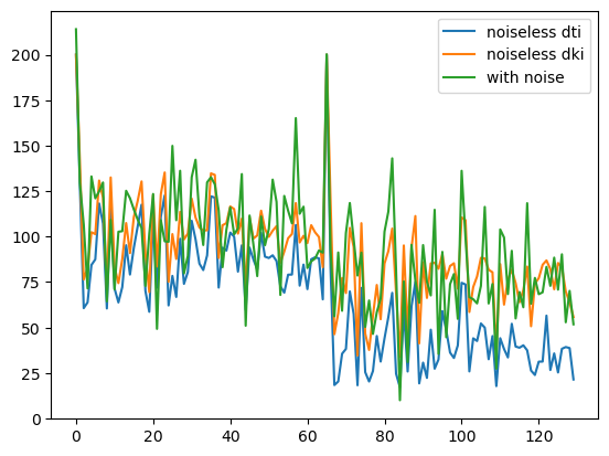
Simulated signals obtain from the DTI and DKI models.

Non-Gaussian diffusion properties in tissues are responsible to smaller signal attenuation for larger bvalues when compared to signal attenuation from free Gaussian water diffusion. This feature can be shown from the figure above, since signals simulated from the DKI models reveals larger DW signal intensities than the signals obtained only from the diffusion tensor components.

References

[RNH2015]

R. Neto Henriques et al., “Exploring the 3D geometry of the diffusion kurtosis tensor - Impact on the development of robust tractography procedures and novel biomarkers”, NeuroImage (2015) 111, 85-99.