Noise estimation using PIESNO

Often, one is interested in estimating the noise in the diffusion signal. One of the methods to do this is the Probabilistic Identification and Estimation of Noise (PIESNO) framework [1]. Using this method, one can detect the standard deviation of the noise from Diffusion-Weighted Imaging (DWI). PIESNO also works with multiple channel DWI datasets that are acquired from N array coils for both SENSE and GRAPPA reconstructions.

The PIESNO method works in two steps:

1) First, it finds voxels that are most likely background voxels. Intuitively, these voxels have very similar diffusion-weighted intensities (up to some noise) in the fourth dimension of the DWI dataset. White matter, gray matter or CSF voxels have diffusion intensities that vary quite a lot across different directions.

2) From these estimated background voxels and the input number of coils \(N\), PIESNO finds what sigma each Gaussian from each of the \(N\) coils would have generated the observed Rician (\(N = 1\)) or non-central Chi (\(N > 1\)) distributed noise profile in the DWI datasets.

PIESNO makes an important assumption: the Gaussian noise standard deviation is assumed to be uniform. The noise is uniform across multiple slice locations or across multiple images of the same location.

For the full details, please refer to the original paper.

In this example, we will demonstrate the use of PIESNO with a 3-shell data-set.

We start by importing necessary modules and functions:

import matplotlib.pyplot as plt
import numpy as np

from dipy.data import get_fnames
from dipy.denoise.noise_estimate import piesno
from dipy.io.image import load_nifti, save_nifti

Then we load the data and the affine:

dwi_fname, dwi_bval_fname, dwi_bvec_fname = get_fnames(name="sherbrooke_3shell")
data, affine = load_nifti(dwi_fname)

Now that we have fetched a dataset, we must call PIESNO with the right number of coils used to acquire this dataset. It is also important to know what was the parallel reconstruction algorithm used. Here, the data comes from a GRAPPA reconstruction, was acquired with a 12-elements head coil available on the Tim Trio Siemens, for which the 12 coil elements are combined into 4 groups of 3 coil elements each. The signal is therefore received through 4 distinct groups of receiver channels, yielding N = 4. Had we used a GE acquisition, we would have used N=1 even if multiple channel coils are used because GE uses a SENSE reconstruction, which has a Rician noise nature and thus N is always 1.

sigma, mask = piesno(data, N=4, return_mask=True)

axial = data[:, :, data.shape[2] // 2, 0].T
axial_piesno = mask[:, :, data.shape[2] // 2].T

fig, ax = plt.subplots(1, 2)
ax[0].imshow(axial, cmap="gray", origin="lower")
ax[0].set_title("Axial slice of the b=0 data")
ax[1].imshow(axial_piesno, cmap="gray", origin="lower")
ax[1].set_title("Background voxels from the data")
for a in ax:
    a.set_axis_off()

plt.savefig("piesno.png", bbox_inches="tight")

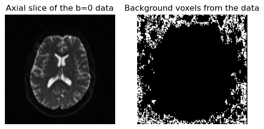
Showing the mid axial slice of the b=0 image (left) and estimated background voxels (right) used to estimate the noise standard deviation.

save_nifti("mask_piesno.nii.gz", mask.astype(np.uint8), affine)

print("The noise standard deviation is sigma = ", sigma)
print("The std of the background is =", np.std(data[mask[..., :].astype(bool)]))

The noise standard deviation is sigma =  [7.263329  7.263329  7.263329  6.933178  7.263329  6.933178  6.933178
 6.933178  6.933178  6.933178  6.933178  7.263329  7.263329  6.933178
 7.5934806 7.263329  7.5934806 7.263329  7.263329  7.263329  7.5934806
 7.263329  7.5934806 7.5934806 7.263329  7.263329  7.5934806 7.5934806
 7.263329  7.263329  7.263329  7.5934806 7.263329  7.263329  7.263329
 7.263329  7.263329  7.263329  7.263329  7.263329  7.263329  7.263329
 7.263329  6.933178  7.263329  6.933178  6.933178  6.933178  6.933178
 6.933178  7.263329  7.263329  7.263329  7.263329  7.263329  7.263329
 7.263329  7.263329  7.263329  7.263329 ]
The std of the background is = 9.708311737182022

Here, we obtained a noise standard deviation of 7.26. For comparison, a simple standard deviation of all voxels in the estimated mask (as done in the previous example SNR estimation for Diffusion-Weighted Images) gives a value of 6.1.

References

[1]

Cheng Guan Koay, Evren Özarslan, and Carlo Pierpaoli. Probabilistic Identification and Estimation of Noise (PIESNO): A self-consistent approach and its applications in MRI. Journal of Magnetic Resonance, 199(1):94–103, July 2009. URL: https://doi.org/10.1016/j.jmr.2009.03.005, doi:10.1016/j.jmr.2009.03.005.