Fast Streamline Search

This example explains how Fast Streamline Search [1] can be used to find all similar streamlines.

First import the necessary modules.

import numpy as np

from dipy.data import (
    fetch_bundle_atlas_hcp842,
    fetch_target_tractogram_hcp,
    get_target_tractogram_hcp,
    get_two_hcp842_bundles,
)
from dipy.io.streamline import load_trk
from dipy.segment.fss import FastStreamlineSearch, nearest_from_matrix_row
from dipy.viz import actor, window

Download and read data for this tutorial

fetch_bundle_atlas_hcp842()
fetch_target_tractogram_hcp()

hcp_file = get_target_tractogram_hcp()
streamlines = load_trk(hcp_file, "same", bbox_valid_check=False).streamlines

Visualize the atlas (ref) bundle and full brain tractogram

interactive = False

scene = window.Scene()
scene.SetBackground(1, 1, 1)
scene.add(actor.line(streamlines))
if interactive:
    window.show(scene)
else:
    window.record(scene=scene, out_path="tractograms_initial.png", size=(600, 600))

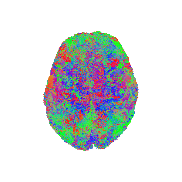
Atlas bundle and source streamlines before registration.

Read Arcuate Fasciculus Left and Corticospinal Tract Left bundles from already fetched atlas data to use them as model bundle. Let’s visualize the Arcuate Fasciculus Left model bundle.

model_af_l_file, model_cst_l_file = get_two_hcp842_bundles()
sft_af_l = load_trk(model_af_l_file, "same", bbox_valid_check=False)
model_af_l = sft_af_l.streamlines

scene = window.Scene()
scene.SetBackground(1, 1, 1)
scene.add(actor.line(model_af_l, colors=(0, 1, 0)))
scene.set_camera(
    focal_point=(-18.17281532, -19.55606842, 6.92485857),
    position=(-360.11, -30.46, -40.44),
    view_up=(-0.03, 0.028, 0.89),
)
if interactive:
    window.show(scene)
else:
    window.record(scene=scene, out_path="AF_L_model_bundle.png", size=(600, 600))

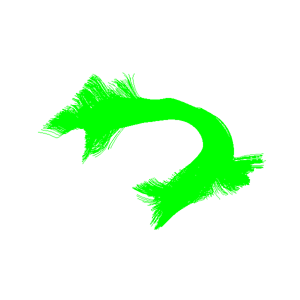
Model Arcuate Fasciculus Left bundle

Search for all similar streamlines [1]

Fast Streamline Search can do a radius search to find all streamlines that are similar to from one tractogram to another. It returns the distance matrix mapping between both tractograms. The same list of streamlines can be given to recover the self distance matrix.

here are the FastStreamlinesSearch class need the following initialization arguments:

• ref_streamlines : reference streamlines, that will be searched in (tree)

• max_radius : is the maximum distance that can be used with radius search

Then, the radius_search() method needs the following arguments:

• radius : for each streamline search find all similar ones in the “ref_streamlines” that are within the given radius

Be cautious, a large radius might result in a dense distance computation, requiring a large amount of time and memory. Recommended range of the radius is from 1 to 10 mm.

radius = 7.0
fs_tree_af = FastStreamlineSearch(ref_streamlines=model_af_l, max_radius=radius)
coo_mdist_mtx = fs_tree_af.radius_search(streamlines, radius=radius)

Extract indices of streamlines with an similar ones in the reference

ids_s = np.unique(coo_mdist_mtx.row)
ids_ref = np.unique(coo_mdist_mtx.col)

recognized_af_l = streamlines[ids_s].copy()

let’s visualize streamlines similar to the Arcuate Fasciculus Left bundle

scene = window.Scene()
scene.SetBackground(1, 1, 1)
scene.add(actor.line(recognized_af_l, colors=(0, 0, 1)))
scene.set_camera(
    focal_point=(-18.17281532, -19.55606842, 6.92485857),
    position=(-360.11, -30.46, -40.44),
    view_up=(-0.03, 0.028, 0.89),
)
if interactive:
    window.show(scene)
else:
    window.record(scene=scene, out_path="AF_L_recognized_bundle.png", size=(600, 600))

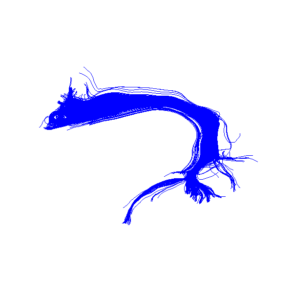
Recognized Arcuate Fasciculus Left bundle

Color the resulting AF by the nearest streamlines distance

nn_s, nn_ref, nn_dist = nearest_from_matrix_row(coo_mdist_mtx)

scene = window.Scene()
scene.SetBackground(1, 1, 1)
cmap = actor.colormap_lookup_table(scale_range=(nn_dist.min(), nn_dist.max()))
scene.add(actor.line(recognized_af_l, colors=nn_dist, lookup_colormap=cmap))
scene.add(actor.scalar_bar(lookup_table=cmap, title="distance to atlas (mm)"))
scene.set_camera(
    focal_point=(-18.17281532, -19.55606842, 6.92485857),
    position=(-360.11, -30.46, -40.44),
    view_up=(-0.03, 0.028, 0.89),
)
if interactive:
    window.show(scene)
else:
    window.record(
        scene=scene, out_path="AF_L_recognized_bundle_dist.png", size=(600, 600)
    )

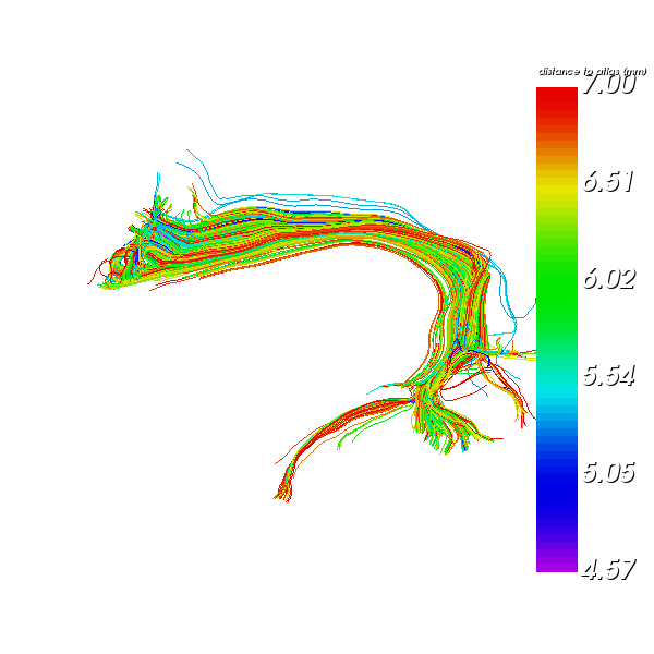
Recognized Arcuate Fasciculus Left bundle colored by distance to ref

Display the streamlines reference reached in green

# Default red color
ref_color = np.zeros((len(model_af_l), 3), dtype=float)
ref_color[:] = (1.0, 0.0, 0.0)

# Reached in green color
ref_color[ids_ref] = (0.0, 1.0, 0.0)

scene = window.Scene()
scene.SetBackground(1, 1, 1)
scene.add(actor.line(model_af_l, colors=ref_color))
scene.set_camera(
    focal_point=(-18.17281532, -19.55606842, 6.92485857),
    position=(-360.11, -30.46, -40.44),
    view_up=(-0.03, 0.028, 0.89),
)

if interactive:
    window.show(scene)
else:
    window.record(
        scene=scene, out_path="AF_L_model_bundle_reached.png", size=(600, 600)
    )

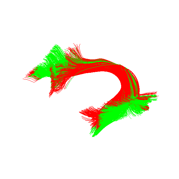
Arcuate Fasciculus Left model reached (green) in radius

References

[1] (1,2)

Etienne St-Onge, Eleftherios Garyfallidis, and D. Louis Collins. Fast Streamline Search: An Exact Technique for Diffusion MRI Tractography. Neuroinformatics, 20(4):1093–1104, 2022. URL: https://doi.org/10.1007/s12021-022-09590-7, doi:10.1007/s12021-022-09590-7.