Calculate SHORE scalar maps

We show how to calculate two SHORE-based scalar maps: return to origin probability (RTOP) [Descoteaux2011] and mean square displacement (MSD) [Wu2007], [Wu2008] on your data. SHORE can be used with any multiple b-value dataset like multi-shell or DSI.

First import the necessary modules:

import numpy as np
import matplotlib.pyplot as plt
from dipy.core.gradients import gradient_table
from dipy.data import get_fnames
from dipy.io.gradients import read_bvals_bvecs
from dipy.io.image import load_nifti
from dipy.reconst.shore import ShoreModel

Download and get the data filenames for this tutorial.

fraw, fbval, fbvec = get_fnames('taiwan_ntu_dsi')

img contains a nibabel Nifti1Image object (data) and gtab contains a GradientTable object (gradient information e.g. b-values). For example, to read the b-values it is possible to write print(gtab.bvals).

Load the raw diffusion data and the affine.

data, affine = load_nifti(fraw)
bvals, bvecs = read_bvals_bvecs(fbval, fbvec)
bvecs[1:] = (bvecs[1:] /
             np.sqrt(np.sum(bvecs[1:] * bvecs[1:], axis=1))[:, None])
gtab = gradient_table(bvals, bvecs)
print('data.shape (%d, %d, %d, %d)' % data.shape)

data.shape (96, 96, 60, 203)

Instantiate the Model.

asm = ShoreModel(gtab)

Let’s just use only one slice only from the data.

dataslice = data[30:70, 20:80, data.shape[2] // 2]

Fit the signal with the model and calculate the SHORE coefficients.

asmfit = asm.fit(dataslice)

  0%|                                                                                                                                          | 0/2400 [00:00<?, ?it/s]C:\Users\skoudoro\Devel\dipy\dipy\core\geometry.py:130: RuntimeWarning: invalid value encountered in arccos
  theta = np.arccos(np.divide(z, r, where=r > 0))

  0%|                                                                                                                                  | 1/2400 [00:00<06:41,  5.98it/s]
  6%|███████▉                                                                                                                       | 151/2400 [00:00<00:03, 691.41it/s]
 13%|███████████████▉                                                                                                              | 304/2400 [00:00<00:02, 1022.22it/s]
 19%|███████████████████████▉                                                                                                      | 455/2400 [00:00<00:01, 1196.99it/s]
 25%|███████████████████████████████▉                                                                                              | 608/2400 [00:00<00:01, 1308.83it/s]
 32%|████████████████████████████████████████                                                                                      | 764/2400 [00:00<00:01, 1387.29it/s]
 38%|████████████████████████████████████████████████                                                                              | 915/2400 [00:00<00:01, 1424.78it/s]
 44%|███████████████████████████████████████████████████████▋                                                                     | 1068/2400 [00:00<00:00, 1456.23it/s]
 51%|███████████████████████████████████████████████████████████████▌                                                             | 1220/2400 [00:00<00:00, 1474.55it/s]
 57%|███████████████████████████████████████████████████████████████████████▎                                                     | 1370/2400 [00:01<00:00, 1476.43it/s]
 63%|███████████████████████████████████████████████████████████████████████████████▎                                             | 1522/2400 [00:01<00:00, 1488.35it/s]
 70%|███████████████████████████████████████████████████████████████████████████████████████                                      | 1672/2400 [00:01<00:00, 1481.71it/s]
 76%|███████████████████████████████████████████████████████████████████████████████████████████████▍                             | 1833/2400 [00:01<00:00, 1520.02it/s]
 83%|███████████████████████████████████████████████████████████████████████████████████████████████████████▍                     | 1986/2400 [00:01<00:00, 1515.18it/s]
 89%|███████████████████████████████████████████████████████████████████████████████████████████████████████████████▎             | 2138/2400 [00:01<00:00, 1515.25it/s]
 95%|███████████████████████████████████████████████████████████████████████████████████████████████████████████████████████▎     | 2290/2400 [00:01<00:00, 1513.11it/s]
100%|█████████████████████████████████████████████████████████████████████████████████████████████████████████████████████████████| 2400/2400 [00:01<00:00, 1370.41it/s]

Calculate the analytical RTOP on the signal that corresponds to the integral of the signal.

print('Calculating... rtop_signal')
rtop_signal = asmfit.rtop_signal()

Calculating... rtop_signal

Now we calculate the analytical RTOP on the propagator, that corresponds to its central value.

print('Calculating... rtop_pdf')
rtop_pdf = asmfit.rtop_pdf()

Calculating... rtop_pdf

In theory, these two measures must be equal, to show that we calculate the mean square error on this two measures.

mse = np.sum((rtop_signal - rtop_pdf) ** 2) / rtop_signal.size
print(f"MSE = {mse:f}")

MSE = 0.000000

Let’s calculate the analytical mean square displacement on the propagator.

print('Calculating... msd')
msd = asmfit.msd()

Calculating... msd

Show the maps and save them to a file.

fig = plt.figure(figsize=(6, 6))
ax1 = fig.add_subplot(2, 2, 1, title='rtop_signal')
ax1.set_axis_off()
ind = ax1.imshow(rtop_signal.T, interpolation='nearest', origin='lower')
plt.colorbar(ind)
ax2 = fig.add_subplot(2, 2, 2, title='rtop_pdf')
ax2.set_axis_off()
ind = ax2.imshow(rtop_pdf.T, interpolation='nearest', origin='lower')
plt.colorbar(ind)
ax3 = fig.add_subplot(2, 2, 3, title='msd')
ax3.set_axis_off()
ind = ax3.imshow(msd.T, interpolation='nearest', origin='lower', vmin=0)
plt.colorbar(ind)
plt.savefig('SHORE_maps.png')

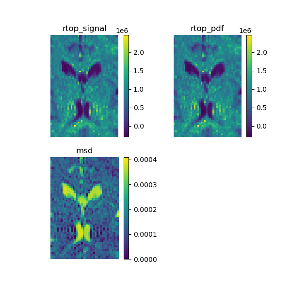
RTOP and MSD calculated using the SHORE model.

References

[Descoteaux2011]

Descoteaux M. et al., “Multiple q-shell diffusion propagator imaging”, Medical Image Analysis, vol 15, No. 4, p. 603-621, 2011.

[Wu2007]

Wu Y. et al., “Hybrid diffusion imaging”, NeuroImage, vol 36, p. 617-629, 2007.

[Wu2008]

Wu Y. et al., “Computation of Diffusion Function Measures in q-Space Using Magnetic Resonance Hybrid Diffusion Imaging”, IEEE TRANSACTIONS ON MEDICAL IMAGING, vol. 27, No. 6, p. 858-865, 2008.