Interactive Visualization with DIPY Horizon (Python)

This tutorial demonstrates how to use DIPY Horizon programmatically in Python code for interactive visualization of tractography data, brain images, surfaces, and peak directions. Horizon is a powerful interactive medical visualization tool introduced in Garyfallidis et al.[1].

While Horizon can be used from the command line (see dMRI Visualization with Horizon), this example shows how to use it directly in Python scripts for more flexible and programmatic visualization workflows.

What is Horizon?

Horizon is DIPY’s interactive visualization system that allows you to:

• Visualize and interact with tractograms (streamlines)

• Display anatomical images (T1, T2, FA, etc.) as slices

• Cluster streamlines using QuickBundlesX

• Visualize peak directions and spherical harmonics

• Display brain surfaces (cortical meshes)

• Combine multiple data types in a single view

• Save snapshots of your visualizations

Getting Started

First, let’s import the necessary modules and check that we have FURY installed (required for 3D visualization):

import sys

import numpy as np

from dipy.core.gradients import gradient_table
from dipy.data import default_sphere, get_fnames
from dipy.direction import peaks_from_model
from dipy.io.gradients import read_bvals_bvecs
from dipy.io.image import load_nifti
from dipy.io.stateful_tractogram import Space, StatefulTractogram
from dipy.reconst.csdeconv import (
    ConstrainedSphericalDeconvModel,
    auto_response_ssst,
)
from dipy.reconst.dti import TensorModel
from dipy.segment.mask import median_otsu
from dipy.tracking import utils
from dipy.tracking.stopping_criterion import ThresholdStoppingCriterion
from dipy.tracking.streamline import Streamlines
from dipy.tracking.tracker import deterministic_tracking
from dipy.utils.logging import logger
from dipy.utils.optpkg import optional_package

fury, has_fury, setup_module = optional_package("fury")

interactive = False  # Set to True for interactive visualization!

# Check if FURY is available
if not has_fury:
    logger.error("FURY is required for Horizon. Install it with: pip install fury")
    sys.exit(1)

from dipy.viz import horizon

Basic Example: Visualizing a Brain Image

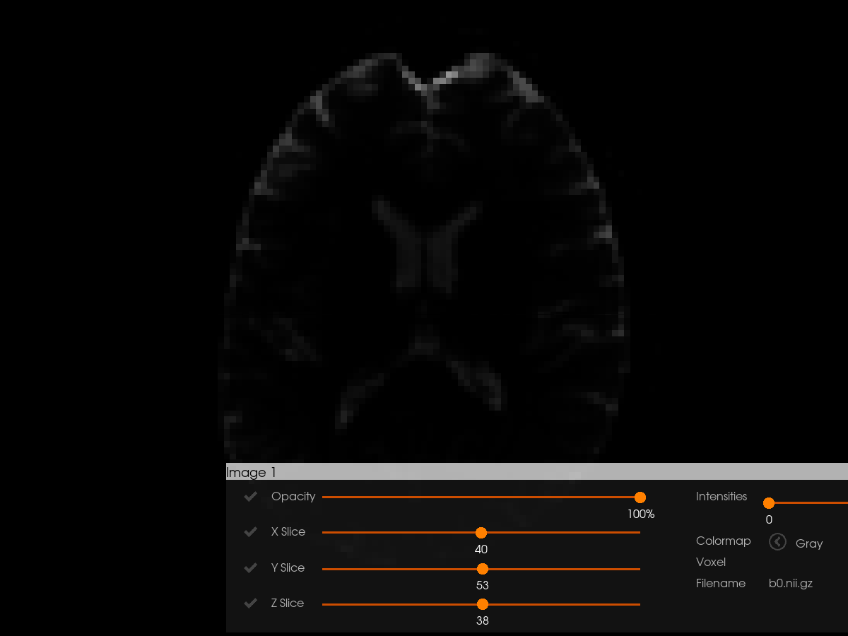
Let’s start with the simplest use case: visualizing a 3D brain image. Load example diffusion data (Stanford HARDI) We’ll extract and visualize its b0 volume (first 3D volume of the 4D data).

# Load example data
hardi_fname, hardi_bval_fname, hardi_bvec_fname = get_fnames(name="stanford_hardi")
data, affine, hardi_img = load_nifti(hardi_fname, return_img=True)

# Extract the first b0 image (this dataset has multiple b0 volumes)
b0_data = data[..., 0]

To visualize an image with Horizon, we need to provide it as a tuple containing (data, affine, optional_filename). The affine matrix defines the spatial orientation of the image.

# Prepare image data for Horizon
images = [(b0_data, affine, "b0.nii.gz")]

# Create visualization
horizon(
    images=images,
    world_coords=True,  # Use world coordinates (not voxel coordinates)
    interactive=interactive,  # Controlled by flag at top of script
    out_png="horizon_basic_image.png",
)

if not interactive:
    logger.info("Saved: horizon_basic_image.png")

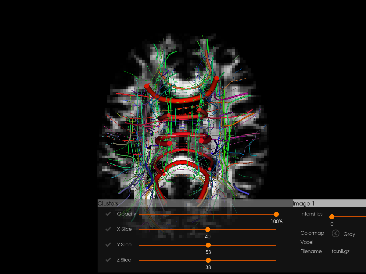
Visualizing Tractograms with Clustering

One of Horizon’s most powerful features is interactive tractography visualization with automatic clustering using QuickBundlesX.

# Create FA map and white matter mask for tractography
bvals, bvecs = read_bvals_bvecs(hardi_bval_fname, hardi_bvec_fname)
gtab = gradient_table(bvals, bvecs=bvecs)

# Create white matter mask first
_, white_matter_mask = median_otsu(data, vol_idx=range(10, 50), numpass=3)

logger.info("Computing tensor model...")
tenmodel = TensorModel(gtab)
tenfit = tenmodel.fit(data, mask=white_matter_mask)
fa_data = tenfit.fa

logger.info("Generating streamlines...")

# Create seeds
seeds = utils.seeds_from_mask(white_matter_mask, affine, density=[2, 2, 2])
# Use a subset of seeds for faster demo execution
np.random.shuffle(seeds)
seeds = seeds[:5000]

# Create stopping criterion from FA
stopping_criterion = ThresholdStoppingCriterion(fa_data, 0.2)

# Perform tractography using the modern functional tracker
# Build a CSD model to get SH coefficients for deterministic tracking
logger.info("Computing CSD model...")
response, _ = auto_response_ssst(gtab, data, roi_radii=10, fa_thr=0.7)
csd_model = ConstrainedSphericalDeconvModel(gtab, response, sh_order_max=6)
csd_fit = csd_model.fit(data, mask=white_matter_mask)

# Generate streamlines with built-in length filtering
# min_len and max_len filter during tracking (no post-processing needed)
streamline_generator = deterministic_tracking(
    seeds,
    stopping_criterion,
    affine,
    step_size=0.5,
    min_len=10,  # Minimum length in mm (filters short streamlines)
    max_len=500,  # Maximum length in mm
    sh=csd_fit.shm_coeff,
    max_angle=30.0,
    sphere=default_sphere,
    nbr_threads=0,  # 0 = auto-detect cores; set to >0 for explicit threading
    return_all=False,
)

streamlines = Streamlines(streamline_generator)
logger.info(f"Generated {len(streamlines)} streamlines (min_len=10mm, max_len=500mm)")

# Create StatefulTractogram (required for Horizon)
# Using the image object directly ensures proper coordinate system handling
sft = StatefulTractogram(streamlines, hardi_img, Space.RASMM)

Now visualize with clustering enabled. Clustering groups similar streamlines together, making it easier to explore large tractography datasets. We also overlay the tractography on FA for anatomical context.

tractograms = [sft]

horizon(
    tractograms=tractograms,
    images=[(fa_data, affine, "fa.nii.gz")],
    cluster=True,  # Enable QuickBundlesX clustering
    cluster_thr=15.0,  # Distance threshold in mm
    length_gt=30,  # Filter: show streamlines > 30mm
    length_lt=150,  # Filter: show streamlines < 150mm
    clusters_gt=10,  # Filter: show clusters with > 10 streamlines
    world_coords=True,
    interactive=interactive,
    out_png="horizon_tractography.png",
)

if not interactive:
    logger.info("Saved: horizon_tractography.png")

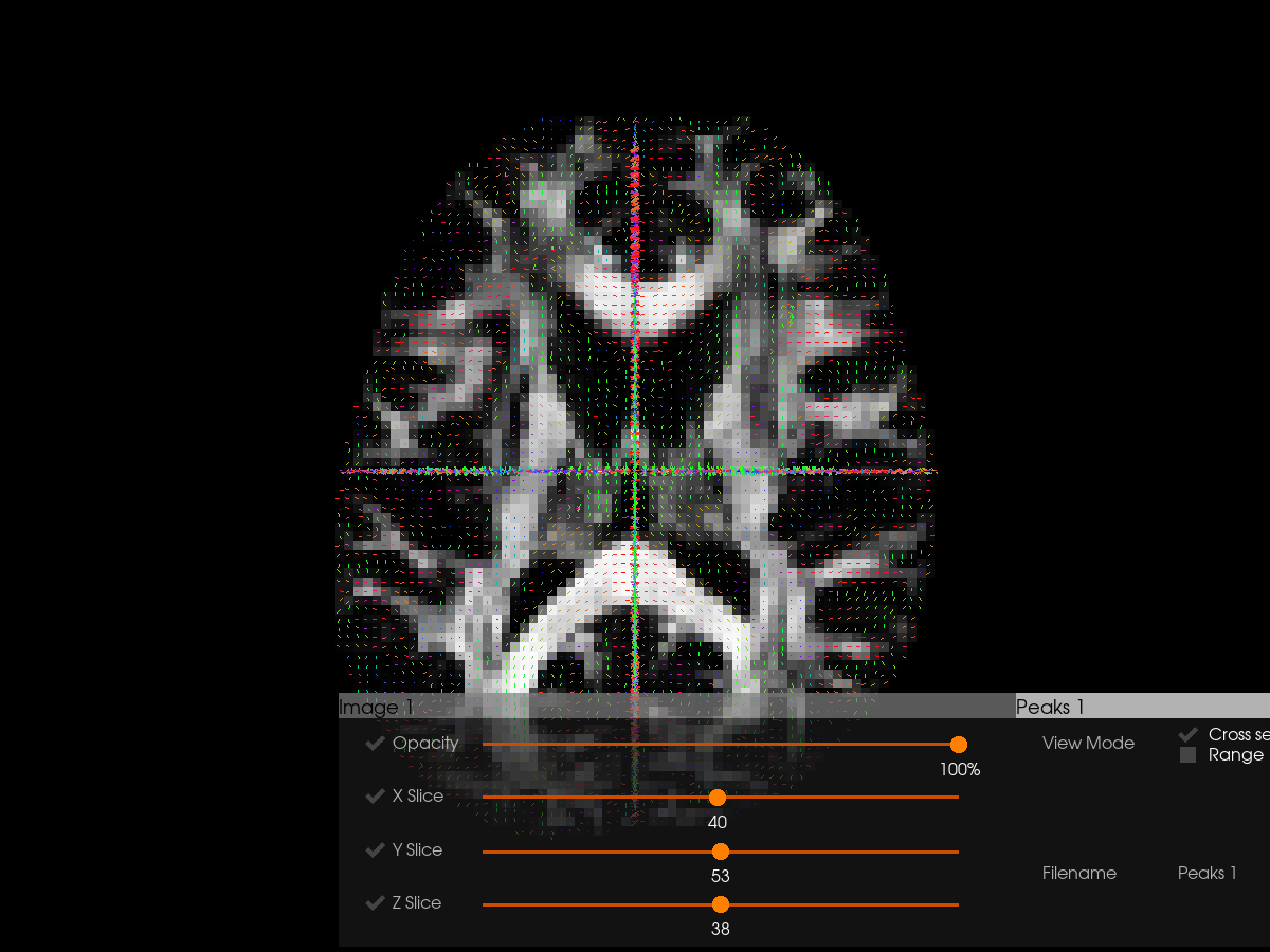
Visualizing Peak Directions

logger.info("Computing peaks...")

# Compute peaks from the tensor model using the white matter mask
dti_peaks = peaks_from_model(
    tenmodel,
    data,
    default_sphere,
    relative_peak_threshold=0.5,
    min_separation_angle=25,
    mask=white_matter_mask,
)

# Add affine to peaks for visualization
dti_peaks.affine = affine

# Visualize peaks with FA background
horizon(
    pams=[dti_peaks],
    images=[(fa_data, affine, "fa.nii.gz")],
    world_coords=True,
    interactive=interactive,
    out_png="horizon_dti_peaks.png",
)

if not interactive:
    logger.info("Saved: horizon_dti_peaks.png")

Interactive Mode

All the examples above use interactive=False to automatically save images. For actual data exploration, set interactive=True to open an interactive window where you can:

• Left click: select clusters

• E: expand clusters

• R: collapse all clusters

• H: hide unselected clusters

• I: invert selection

• A: select all clusters

• S: save selected streamlines to file

• Y: open new window

• O: hide/show control panel

Mouse controls:

• Shift + drag: move camera

• Ctrl/Cmd + drag: rotate camera

• Ctrl/Cmd + R: reset camera

Note: The window will stay open until you close it manually.

Summary

This tutorial covered:

1. Basic image visualization with Horizon

2. Visualizing tractography with clustering and filtering

3. Visualizing peak directions

4. Interactive exploration with keyboard/mouse controls

Key Parameters Summary

• tractograms: List of StatefulTractogram objects

• images: List of tuples (data, affine, filename)

• pams: List of PeakAndMetrics objects

• surfaces: List of tuples (vertices, faces, filename)

• cluster: Enable QuickBundlesX clustering (bool)

• cluster_thr: Distance threshold for clustering in mm (float)

• length_gt/length_lt: Filter streamlines by length (float)

• clusters_gt/clusters_lt: Filter by cluster size (int)

• world_coords: Use world coordinates vs voxel coordinates (bool)

• interactive: Enable interactive window (bool)

• out_png: Output filename for snapshot (str)

• bg_color: Background color as RGB tuple (tuple)

• roi_images: Display images as ROI contours (bool)

• random_colors: Use random colors for tractograms/ROIs (str or bool)

For more details, see the Horizon documentation and the command-line interface tutorial at dMRI Visualization with Horizon.

See [1] for further details about Horizon.

References

[1] (1,2)

Eleftherios Garyfallidis, Marc-Alexandre Côté, Bramsh Qamar Chandio, Shreyas Fadnavis, Javier Guaje, Ranveer Aggarwal, Etienne St-Onge, Karandeep Singh Juneja, Serge Koudoro, and David Reagan. DIPY Horizon: fast, modular, unified and adaptive visualization. In ISMRM 27th Annual Meeting & Exhibition SMRT 28th Annual Meeting, volume. Montréal, Canada, 2019. International Society for Magnetic Resonance in Medicine (ISMRM).